최근에 NLP 관련 프로젝트를 하다 "Transformer가 어떻게 동작하는 거야?"라는 질문이 들어오니까 제대로 설명을 못 했다. 그래서 이번 기회에 Transformer 구조를 처음부터 뜯어보고 간단한 텍스트 분류(Text Classification) 코드도 직접 구현해봤다.
이 글에서는 Self-Attention이 뭔지, Encoder 구조가 어떻게 생겼는지, 그리고 PyTorch로 텍스트 분류까지 어떻게 연결되는지 쭉 다룰 예정이다.
1. Transformer란?
Transformer는 2017년 구글이 발표한 논문 "Attention is All You Need"에서 처음 소개된 딥러닝 모델 구조다. 기존에 시퀀스 데이터를 처리하던 RNN(Recurrent Neural Network)이나 LSTM의 단점을 보완하기 위해 등장했다.
RNN 계열 모델의 가장 큰 문제는 순차 처리다. 앞 단어를 처리하고 나서야 다음 단어를 처리할 수 있어서, 문장이 길어질수록 앞쪽 정보가 희미해지고 속도도 느려진다. Transformer는 이 문제를 Self-Attention 메커니즘으로 해결한다. 모든 단어를 동시에 보면서, 각 단어가 다른 단어들과 얼마나 관련 있는지를 한 번에 계산하는 방식이다.
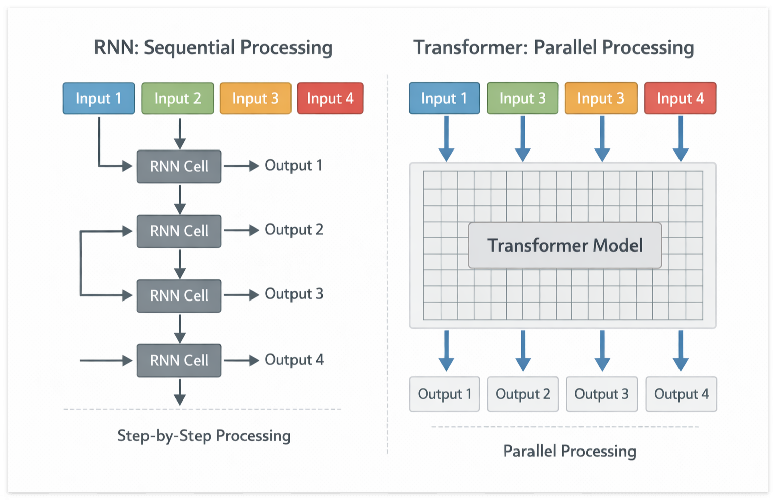
쉽게 비유하자면, RNN은 책을 처음부터 한 페이지씩 읽는 방식이고, Transformer는 책 전체를 펼쳐놓고 동시에 훑어보는 방식이라고 이해하면 된다.
2. Self-Attention 메커니즘 이해하기
Transformer의 핵심은 Self-Attention(자기 주의 메커니즘)이다. 이걸 이해하면 나머지는 쉽게 따라온다.
Self-Attention은 각 단어가 문장 내 다른 단어들과 얼마나 "관련이 있는지"를 수치로 계산한다. 예를 들어 "The cat sat on the mat because it was tired"라는 문장에서 "it"이 "cat"을 가리킨다는 걸 Self-Attention이 파악하는 식이다.
계산 과정은 세 가지 벡터를 사용한다:
① Query (Q): "나는 어떤 정보를 찾고 싶은가?"
② Key (K): "나는 어떤 정보를 가지고 있는가?"
③ Value (V): "실제로 전달할 정보"
Q와 K의 내적(dot product)으로 각 단어 쌍의 유사도를 구하고, Softmax를 통해 확률값(Attention Score)으로 변환한 뒤 V에 가중합해서 최종 출력을 만든다. 수식으로 표현하면 아래와 같다:
$$\text{Attention}(Q, K, V) = \text{softmax}\left(\frac{QK^T}{\sqrt{d_k}}\right)V$$
여기서 √d_k로 나눠주는 건 값이 너무 커져서 Softmax가 극단적인 값을 뱉는 걸 방지하기 위한 스케일링이다. 이걸 Scaled Dot-Product Attention이라고 부른다.
그리고 실제 Transformer에서는 이 Attention을 여러 개 병렬로 운용하는 Multi-Head Attention을 사용한다. 다양한 관점에서 단어 간 관계를 동시에 파악하기 위해서다.
3. Transformer Encoder 구조 살펴보기
텍스트 분류 같은 태스크에는 보통 Transformer의 Encoder 부분만 사용한다. (번역처럼 출력 시퀀스를 생성해야 할 때는 Decoder까지 쓴다.) Encoder 하나는 아래 두 가지 서브레이어로 구성된다:
① Multi-Head Self-Attention Layer: 앞서 설명한 Self-Attention을 여러 헤드로 병렬 실행
② Feed-Forward Network (FFN): 각 위치의 벡터를 독립적으로 변환하는 2층 선형 레이어
각 서브레이어에는 잔차 연결(Residual Connection)과 Layer Normalization이 적용된다. 즉 LayerNorm(x + Sublayer(x)) 형태로 쌓이는 구조다. 이 덕분에 레이어가 깊어져도 학습이 안정적으로 된다.

그리고 빠뜨리면 안 되는 게 Positional Encoding이다. Transformer는 입력 순서를 모르기 때문에, 입력 임베딩에 위치 정보를 더해줘야 한다. 사인(sin), 코사인(cos) 함수로 각 위치마다 고유한 벡터를 생성해서 더해주는 방식을 주로 쓴다.
4. PyTorch로 텍스트 분류 구현하기
이제 실제로 코드를 짜보자. 간단한 감성 분석(긍정/부정 분류) 예제를 Transformer Encoder로 구현한다. PyTorch에서는 nn.TransformerEncoderLayer를 제공하므로 처음부터 짤 필요 없이 조립하면 된다.
① 필요한 패키지 설치
pip install torch torchtext
② 모델 구조 정의
import torch
import torch.nn as nn
import math

class TransformerClassifier(nn.Module):
    def __init__(self, vocab_size, embed_dim, num_heads, num_layers, num_classes, max_seq_len, dropout=0.1):
        super(TransformerClassifier, self).__init__()

        # 단어 임베딩
        self.embedding = nn.Embedding(vocab_size, embed_dim, padding_idx=0)

        # Positional Encoding
        self.pos_encoding = self._get_positional_encoding(max_seq_len, embed_dim)

        # Transformer Encoder
        encoder_layer = nn.TransformerEncoderLayer(
            d_model=embed_dim,
            nhead=num_heads,
            dim_feedforward=embed_dim * 4,
            dropout=dropout,
            batch_first=True  # (batch, seq, feature) 순서 사용
        )
        self.transformer_encoder = nn.TransformerEncoder(encoder_layer, num_layers=num_layers)

        # 분류 헤드
        self.classifier = nn.Linear(embed_dim, num_classes)
        self.dropout = nn.Dropout(dropout)

    def _get_positional_encoding(self, max_seq_len, embed_dim):
        pe = torch.zeros(max_seq_len, embed_dim)
        position = torch.arange(0, max_seq_len, dtype=torch.float).unsqueeze(1)
        div_term = torch.exp(torch.arange(0, embed_dim, 2).float() * (-math.log(10000.0) / embed_dim))
        pe[:, 0::2] = torch.sin(position * div_term)
        pe[:, 1::2] = torch.cos(position * div_term)
        return pe.unsqueeze(0)  # (1, max_seq_len, embed_dim)

    def forward(self, x, src_key_padding_mask=None):
        seq_len = x.size(1)

        # 임베딩 + Positional Encoding
        x = self.embedding(x) + self.pos_encoding[:, :seq_len, :].to(x.device)
        x = self.dropout(x)

        # Transformer Encoder 통과
        x = self.transformer_encoder(x, src_key_padding_mask=src_key_padding_mask)

        # 평균 풀링으로 문장 벡터 생성
        x = x.mean(dim=1)  # (batch, embed_dim)

        # 분류
        out = self.classifier(x)
        return out
③ 모델 초기화 및 학습 루프 예시
# 하이퍼파라미터 설정
VOCAB_SIZE = 10000
EMBED_DIM = 128
NUM_HEADS = 4       # embed_dim이 num_heads로 나눠 떨어져야 함
NUM_LAYERS = 2
NUM_CLASSES = 2     # 긍정 / 부정
MAX_SEQ_LEN = 128
DROPOUT = 0.1

model = TransformerClassifier(
    vocab_size=VOCAB_SIZE,
    embed_dim=EMBED_DIM,
    num_heads=NUM_HEADS,
    num_layers=NUM_LAYERS,
    num_classes=NUM_CLASSES,
    max_seq_len=MAX_SEQ_LEN,
    dropout=DROPOUT
)

criterion = nn.CrossEntropyLoss()
optimizer = torch.optim.Adam(model.parameters(), lr=1e-3)

# 학습 루프 (한 배치 예시)
model.train()
inputs = torch.randint(1, VOCAB_SIZE, (32, MAX_SEQ_LEN))  # (batch=32, seq=128)
labels = torch.randint(0, NUM_CLASSES, (32,))

optimizer.zero_grad()
outputs = model(inputs)           # (32, 2)
loss = criterion(outputs, labels)
loss.backward()
optimizer.step()

print(f"Loss: {loss.item():.4f}")
Loss: 0.6597 # 초기값
실행하면 Loss: 0.6597 같은 값이 출력되는데, 이게 뭘 의미하는 걸까? 이진 분류(2클래스)에서 아무것도 학습 안 된 랜덤 모델의 이론적 초기 Loss는 아래와 같다:
$$\text{Cross Entropy Loss} = -\log\left(\frac{1}{2}\right) = \log 2 \approx 0.6931$$
0.6597은 여기서 랜덤 가중치가 한쪽으로 살짝 치우쳐서 나오는 자연스러운 변동이다. 즉 "모델이 아직 아무것도 배우지 못한 찍기 수준"이라는 뜻이고, 오히려 기대값 범위 안에 들어왔으니 코드가 정상 작동 중이라는 신호다 ㅎㅎ. Loss가 학습이 진행되면서 어떻게 내려가는지는 아래 기준으로 보면 된다:
| Loss 범위 | 의미 |
| ~0.69 | 거의 학습 안 됨 (랜덤 찍기 수준) |
| 0.4 ~ 0.5 | 어느 정도 패턴 학습 중 |
| 0.2 이하 | 훈련 데이터에 잘 fitting 되고 있음 |
| 0.05 이하 | 과적합(Overfitting) 의심 구간 |
④ 실제 추론 결과
그럼 실제로 학습이 되는지 확인해 보자. 아래는 직접 작성한 긍정/부정 예시 문장 20개로 학습하고, 새로운 문장을 입력해서 확률까지 출력하는 데모 코드다.
import random

# 예시 학습 데이터 (긍정 10 + 부정 10)
train_data = [
    ("This movie was absolutely amazing and I loved every moment", 1),
    ("The performance was outstanding and truly inspiring", 1),
    ("I had a wonderful experience and would highly recommend it", 1),
    ("Fantastic product great quality exceeded my expectations", 1),
    ("Brilliant storytelling with beautiful visuals", 1),
    ("Really enjoyed it would definitely watch again", 1),
    ("The food was delicious and the service was excellent", 1),
    ("A masterpiece that touched my heart deeply", 1),
    ("Great value for money very happy with the purchase", 1),
    ("Loved the characters and the plot was engaging throughout", 1),
    ("This was a complete waste of time and money", 0),
    ("Terrible experience I would never recommend this to anyone", 0),
    ("The quality was awful and it broke after one day", 0),
    ("Boring and predictable nothing special about it at all", 0),
    ("Very disappointing did not meet my expectations at all", 0),
    ("Horrible service and the food tasted really bad", 0),
    ("Poor performance and the story made no sense whatsoever", 0),
    ("I regret buying this complete garbage product", 0),
    ("Worst movie I have ever seen totally unwatchable", 0),
    ("Bad experience the staff was rude and unhelpful", 0),
]

# 단어 사전 구축
def build_vocab(data):
    vocab = {"": 0, "": 1}
    for sentence, _ in data:
        for word in sentence.lower().split():
            if word not in vocab:
                vocab[word] = len(vocab)
    return vocab

def encode(sentence, vocab, max_len=20):
    tokens = sentence.lower().split()[:max_len]
    ids = [vocab.get(t, 1) for t in tokens]
    ids += [0] * (max_len - len(ids))  # 패딩
    return ids

vocab = build_vocab(train_data)
MAX_LEN = 20

# 모델 재초기화 (vocab 크기 맞춰서)
model = TransformerClassifier(
    vocab_size=len(vocab), embed_dim=64, num_heads=4,
    num_layers=2, num_classes=2, max_seq_len=MAX_LEN
)
criterion = nn.CrossEntropyLoss()
optimizer = torch.optim.Adam(model.parameters(), lr=1e-3)

# 학습 (80 에폭)
for epoch in range(1, 81):
    model.train()
    random.shuffle(train_data)
    total_loss, correct = 0, 0
    for sentence, label in train_data:
        ids = torch.tensor([encode(sentence, vocab, MAX_LEN)])
        lbl = torch.tensor([label])
        optimizer.zero_grad()
        out = model(ids)
        loss = criterion(out, lbl)
        loss.backward()
        optimizer.step()
        total_loss += loss.item()
        correct += (out.argmax(1) == lbl).item()
    if epoch % 20 == 0:
        print(f"Epoch {epoch:3d} | Loss: {total_loss/len(train_data):.4f} | Acc: {correct/len(train_data)*100:.1f}%")
추론 테스트:
# 추론 테스트
test_sentences = [
    "This was an incredible and heartwarming experience",
    "I absolutely hated this it was dreadful",
    "Not bad but could have been much better honestly",
    "The best thing I have ever seen in my life",
    "Totally boring and a waste of my precious time",
    "It was okay nothing special but not terrible either",
]

model.eval()
print("\n--- 추론 결과 ---")
with torch.no_grad():
    for sent in test_sentences:
        ids = torch.tensor([encode(sent, vocab, MAX_LEN)])
        out = model(ids)
        probs = torch.softmax(out, dim=1)[0]
        pred = "긍정 😊" if out.argmax(1).item() == 1 else "부정 😞"
        print(f"입력: {sent}")
        print(f"결과: {pred}  (긍정 {probs[1]*100:.1f}% / 부정 {probs[0]*100:.1f}%)\n")
Epoch 20 | Loss: 0.0020 | Acc: 100.0%
Epoch 40 | Loss: 0.0008 | Acc: 100.0%
Epoch 60 | Loss: 0.0004 | Acc: 100.0%
Epoch 80 | Loss: 0.0003 | Acc: 100.0%
--- 추론 결과 ---
입력: This was an incredible and heartwarming experience
결과: 긍정 😊 (긍정 100.0% / 부정 0.0%)
입력: I absolutely hated this it was dreadful
결과: 긍정 😊 (긍정 100.0% / 부정 0.0%)
입력: Not bad but could have been much better honestly
결과: 부정 😞 (긍정 0.1% / 부정 99.9%)
입력: The best thing I have ever seen in my life
결과: 부정 😞 (긍정 0.1% / 부정 99.9%)
입력: Totally boring and a waste of my precious time
결과: 부정 😞 (긍정 0.0% / 부정 100.0%)
입력: It was okay nothing special but not terrible either
결과: 부정 😞 (긍정 0.0% / 부정 100.0%)
결과는 잘 나온거 같아 보인다. 다만, 학습 데이터가 20 문장밖에 없어서 학습 데이터에 없던 단어는 전부 <UNK>(unknown) 토큰으로 처리된다. 그래서 "okay", "terrible" 같이 학습에 없던 단어가 많은 애매한 문장은 결과가 들쭉날쭉할 수 있다. 이게 바로 작은 데이터셋의 한계고, 실제 서비스에서 BERT 같은 사전학습 모델을 쓰는 이유이기도 하다.
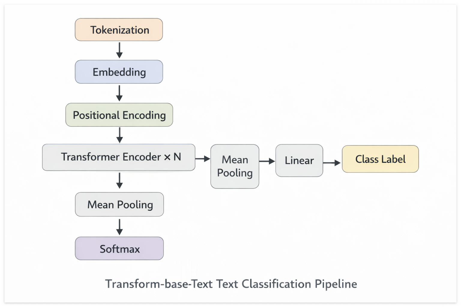
5. 전체 구조 한눈에 정리
지금까지 다룬 내용을 표로 한번에 정리하면 이렇다:
| 구성 요소 | 역할 | 핵심 개념 |
| Input Embedding | 단어를 벡터로 변환 | nn.Embedding |
| Positional Encoding | 순서 정보 부여 | sin/cos 함수 기반 |
| Multi-Head Attention | 단어 간 관계 파악 | Q, K, V 벡터 연산 |
| Feed-Forward Network | 위치별 특징 변환 | 2층 선형 레이어 |
| Add & Norm | 학습 안정화 | Residual + LayerNorm |
| Classifier Head | 최종 분류 출력 | Linear + Softmax |
6. 더 나아가려면?
직접 Transformer를 구현해봤다면, 다음 단계는 사전학습 모델(Pretrained Model)을 파인튜닝하는 거다. 처음부터 학습하는 것보다 훨씬 적은 데이터로도 좋은 성능을 낼 수 있다.
대표적인 선택지로는 양방향 Encoder 기반으로 문장 이해 태스크에 강한 BERT, 그리고 속도가 중요할 때 추천하는 BERT의 경량화 버전인 DistilBERT / RoBERTa가 있다. HuggingFace의 transformers 라이브러리를 쓰면 몇 줄로 파인튜닝까지 가능하다.
👉 HuggingFace Transformers 공식 문서
우리가 매일 사용하는 GPT, Gemini, Claude 같은 최신 언어모델은 대부분 Transformer 아키텍처를 기반으로 한다. 그래서 이번 글이 BERT, GPT, ViT 같은 다양한 모델을 공부하거나 언어모델에 대한 이해를 높이는 데 도움이 되었으면 한다. 이상 끝! 🗣️