데이터 분석 머신러닝을 배우다 보면 보통 전처리 → EDA → 스케일링 → 모델 학습 같은 흐름을 익히게 된다. 하지만 실제로는 이 과정을 각각 따로 다루는 것이 아니라 하나의 흐름으로 연결된 파이프라인으로 설계하는 방법을 알아야 한다. 이번 글에서는 scikit-learn의 Pipeline과 ColumnTransformer를 활용해서 전처리부터 예측까지 하나의 객체로 묶는 방법을 다뤄보았다. 레츠꼬 🔧
1. Machine Learning 파이프라인(Pipeline)이란?
ML을 처음 배울 때는 데이터 불러오기 → 결측치 처리 → 스케일링 → 인코딩 → 모델 학습 → 예측을 각각 따로 코딩하는 경우가 많다.
근데 이 방식은 실수가 생기기 쉽고 train 데이터 기준으로만 fit한 전처리를 test에도 동일하게 적용하는 걸 깜빡하면 데이터 누수(Data Leakage)가 발생한다.
예를 들어 이런 흔한 실수가 있다.
# ❌ 잘못된 방법 — Data Leakage 발생
scaler = StandardScaler()
X_train_scaled = scaler.fit_transform(X_train)
X_test_scaled  = scaler.fit_transform(X_test)  # test에 다시 fit → leakage!

# ✅ 올바른 방법
scaler = StandardScaler()
X_train_scaled = scaler.fit_transform(X_train)  # train에만 fit
X_test_scaled  = scaler.transform(X_test)        # test는 transform만
혹시 위에서 뭐가 잘못된건지 눈치 못 챈 사람들은..! 더더욱 파이프라인 설계를 알아야 한다. (힌트: fit_ 여부)
Pipeline은 이걸 자동으로 보장해준다. fit() 호출 시 각 step의 fit_transform이 순서대로 실행되고, predict() 호출 시에는 transform만 적용된다. 개발자가 직접 신경 쓸 필요가 없다.
Pipeline을 사용하는 이유를 정리하면 다음과 같다.
| 장점 | 설명 |
| Data Leakage 방지 | fit은 train에만, transform/predict는 test에 자동 적용. 직접 관리할 필요 없음 |
| 코드 간결화 | 전처리 + 모델을 하나의 객체로 관리. 단계가 늘어도 코드가 복잡해지지 않음 |
| CV / GridSearch 연동 | cross_val_score, GridSearchCV에 pipe를 통째로 넘기면 각 fold마다 전처리까지 재수행 |
| 배포 단순화 | joblib으로 저장 시 전처리 파라미터(μ, σ, OHE 카테고리 등)까지 전부 포함됨 |
| 재현성 | 전체 흐름이 하나의 객체에 캡슐화되어 실험 재현이 쉬움 |
2. 데이터 파악 및 전처리 전략
예시로 Kaggle의 California Housing Prices 데이터셋을 사용해 파이프라인을 구현해보았다.
👉 California Housing Prices — Kaggle 다운로드
데이터는 총 20,640개 행, 10개 컬럼이다. 타겟은 median_house_value이고 회귀 문제이다.
import pandas as pd

df = pd.read_csv('housing.csv')
print(df.shape)          # (20640, 10)
print(df.isnull().sum())
# total_bedrooms    207  ← 결측치 있음
# 나머지 컬럼       0
print(df['ocean_proximity'].value_counts())
# <1H OCEAN    9136
# INLAND       6551
# NEAR OCEAN   2658
# NEAR BAY     2290
# ISLAND          5
파악한 내용을 정리하면: total_bedrooms에 결측치 207개, ocean_proximity는 범주형 5종. 수치형 컬럼과 범주형 컬럼의 전처리 방식이 다르기 때문에 ColumnTransformer로 분리해서 처리해야 한다.
| 컬럼 | 타입 | 결측치 | 처리 방법 |
| longitude / latitude | float | 0 | StandardScaler 정규화 |
| housing_median_age | float | 0 | StandardScaler 정규화 |
| total_rooms / bedrooms | float | 207 (bedrooms) | SimpleImputer(median) → StandardScaler |
| median_income | float | 0 | StandardScaler 정규화 |
| ocean_proximity | str | 0 | SimpleImputer(most_frequent) → OneHotEncoder |
3. Feature Engineering
raw 컬럼을 그대로 쓰기보다 도메인 지식을 활용해 파생 변수를 만들어주면 모델 성능이 올라간다. 이 작업은 train/test split 전에 전체 데이터에 수행해도 leakage가 없다. 단순 사칙연산이라 통계값을 학습하지 않기 때문이다.
# 파생 변수 생성 (split 전에 수행)
df['rooms_per_household'] = df['total_rooms'] / df['households']
df['bedrooms_per_room'] = df['total_bedrooms'] / df['total_rooms']
df['population_per_household'] = df['population'] / df['households']

X = df.drop('median_house_value', axis=1)
y = df['median_house_value']
나중에 feature importance를 보면 알겠지만, population_per_household가 상위 3위 안에 들 만큼 예측력이 높은 피처가 된다. 총 인구수/세대수 같은 raw 값보다 세대당 인구가 주택 가격과 더 직접적인 관계를 가지기 때문이다.
4. Pipeline + ColumnTransformer 구성
여기가ㅏ 핵심 구조다. 수치형과 범주형을 각각 별도의 sub-pipeline으로 처리하고, ColumnTransformer가 이를 가로로 합쳐(hstack) 하나의 행렬로 만들어준다.
from sklearn.model_selection import train_test_split
from sklearn.pipeline import Pipeline
from sklearn.compose import ColumnTransformer
from sklearn.impute import SimpleImputer
from sklearn.preprocessing import StandardScaler, OneHotEncoder
from sklearn.ensemble import GradientBoostingRegressor

num_features = ['longitude','latitude','housing_median_age','total_rooms',
                'total_bedrooms','population','households','median_income',
                'rooms_per_household','bedrooms_per_room','population_per_household']
cat_features = ['ocean_proximity']

X_train, X_test, y_train, y_test = train_test_split(
    X, y, test_size=0.2, random_state=42
)
# X_train: (16512, 13)  X_test: (4128, 13)

# 수치형 sub-pipeline: 결측치 처리 → 정규화
num_transformer = Pipeline([
    ('imputer', SimpleImputer(strategy='median')),
    ('scaler',  StandardScaler()),
])

# 범주형 sub-pipeline: 최빈값 채우기 → OHE
cat_transformer = Pipeline([
    ('imputer', SimpleImputer(strategy='most_frequent')),
    ('onehot',  OneHotEncoder(handle_unknown='ignore')),
])

# ColumnTransformer: 두 파이프라인을 병렬 실행 후 hstack
preprocessor = ColumnTransformer([
    ('num', num_transformer, num_features),  # → (n, 11)
    ('cat', cat_transformer, cat_features),  # → (n, 5)
])                                           # 최종 → (n, 16)

# 전체 Pipeline
pipe = Pipeline([
    ('preprocessor', preprocessor),
    ('model', GradientBoostingRegressor(
        n_estimators=200, learning_rate=0.1, max_depth=4, random_state=42
    ))
])
ColumnTransformer 출력 shape은 수치형 11개 + OHE 5개 = 총 16개 컬럼이 된다. StandardScaler의 정규화 수식은 아래와 같고, μ와 σ는 반드시 X_train 기준으로만 계산된다.
$$z = \frac{x - \mu_{\text{train}}}{\sigma_{\text{train}}}$$
Pipeline이 이걸 자동으로 보장하기 때문에 test set에 train 통계값을 수동으로 적용하는 실수를 원천 차단할 수 있다.
5. 모델 학습 및 비교
같은 preprocessor를 공유하면서 모델만 바꿔가며 Ridge, RandomForest, GradientBoosting 세 가지를 비교했다. Pipeline을 쓰면 모델 교체가 마지막 step 한 줄 수정으로 끝난다.
import numpy as np
from sklearn.linear_model import Ridge
from sklearn.ensemble import RandomForestRegressor, GradientBoostingRegressor
from sklearn.model_selection import cross_val_score
from sklearn.metrics import mean_squared_error, mean_absolute_error, r2_score

models = {
    'Ridge':            Ridge(alpha=1.0),
    'RandomForest':     RandomForestRegressor(n_estimators=100, random_state=42, n_jobs=-1),
    'GradientBoosting': GradientBoostingRegressor(
                            n_estimators=200, learning_rate=0.1,
                            max_depth=4, random_state=42),
}

for name, model in models.items():
    pipe = Pipeline([('preprocessor', preprocessor), ('model', model)])
    pipe.fit(X_train, y_train)
    y_pred = pipe.predict(X_test)

    rmse = np.sqrt(mean_squared_error(y_test, y_pred))
    mae  = mean_absolute_error(y_test, y_pred)
    r2   = r2_score(y_test, y_pred)
    cv   = cross_val_score(pipe, X_train, y_train,
                           cv=5, scoring='neg_root_mean_squared_error', n_jobs=-1)
    print(f"{name}: RMSE=${rmse:,.0f}  MAE=${mae:,.0f}  R²={r2:.4f}  CV=${-cv.mean():,.0f}±{cv.std():,.0f}")

| 모델 | RMSE | MAE | R² | 5-fold CV RMSE |
| Ridge | $69,135 | $49,652 | 0.6353 | $67,848 ± $1,564 |
| RandomForest | $49,834 | $31,926 | 0.8105 | $50,216 ± $659 |
| GradientBoosting ✅ | $48,287 | $32,234 | 0.8221 | $48,230 ± $941 |
GradientBoosting이 RMSE $48,287, R² 0.8221로 가장 좋은 성능을 냈다. 주목할 점은 CV RMSE ($48,230)와 Test RMSE ($48,287)가 거의 동일하다는 것이다. 이는 Pipeline 덕분에 각 CV fold마다 전처리가 올바르게 재수행되어, 과적합 없이 일반화가 잘 되고 있다는 신호다.
+ RMSE, MAE, 그리고 교차검증 기반 RMSE는 단순한 숫자가 아니라 타겟 변수와 동일한 단위($)를 가지므로 실제 오차의 크기를 직관적으로 해석할 수 있다.
GradientBoosting이 RandomForest보다 나은 이유는 잔차(residual)를 반복적으로 보정하는 boosting 구조 때문이다. 수식으로 표현하면 m번째 트리는 이전까지의 잔차를 학습한다.
$$F_m(x) = F_{m-1}(x) + \eta \cdot h_m(x)$$
여기서 $$\eta$$는 learning_rate(0.1), $$h_m$$은 m번째 약한 학습기(weak learner)다. learning_rate가 낮을수록 각 트리의 기여를 줄여 과적합을 방지하지만, 그만큼 더 많은 n_estimators가 필요하다.
6. 피처 중요도(Feature Importances) & 예측 품질 분석
GradientBoosting의 feature_importances_를 뽑아보면 median_income 하나가 전체 variance의 53%를 설명하고 있다. Pipeline 내부의 각 step에는 named_steps로 접근할 수 있다.
# Pipeline 내부 step에 접근하기
ohe_cats = (pipe.named_steps['preprocessor']
               .named_transformers_['cat']['onehot']
               .get_feature_names_out(['ocean_proximity']))

all_features = num_features + list(ohe_cats)
importances  = pipe.named_steps['model'].feature_importances_

feat_imp_df = (pd.DataFrame({'feature': all_features, 'importance': importances})
                 .sort_values('importance', ascending=False))
print(feat_imp_df.head(5))

#              feature  importance
#        median_income    0.530612
# ocean_proximity_INLAND 0.147924
# population_per_household 0.113864
#            longitude    0.070490
#             latitude    0.058693

Actual vs Predicted scatter를 보면 저가~중가 구간은 예측이 잘 모이지만, $400k 이상 고가 구간에서 분산이 커지는 경향이 있다. 이 데이터셋은 상한선이 $500,001로 캡핑되어 있어서 모델 입장에서는 해당 구간의 진짜 가격을 알 수 없기 때문이다. 실제 서비스라면 이 구간을 별도로 처리하거나, 캡핑이 없는 데이터를 추가 수집하는 게 필요하다.
7. 잔차 분석 및 세그먼트별 성능
잔차(residual)를 분석하면 모델의 체계적 오류 패턴을 잡을 수 있다. 잔차 정의는 아래와 같다.
$$e_i = y_i - \hat{y}_i$$
좋은 회귀 모델이라면 잔차가 0 주변에 무작위(homoscedastic)로 분포해야 한다. 특정 예측값 구간에서 잔차가 한쪽으로 치우치거나 분산이 커지는 이분산성(heteroscedasticity)이 보이면 모델이 해당 구간에서 체계적으로 틀리고 있다는 신호다.
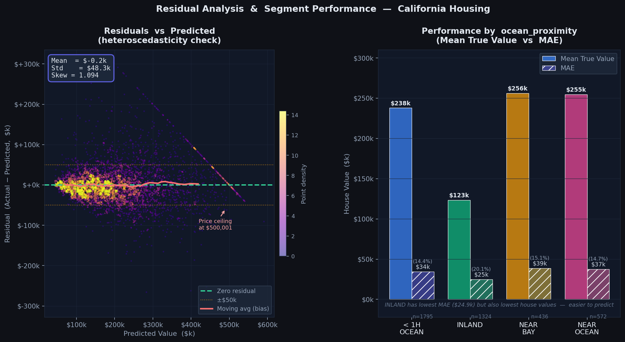
ocean_proximity별로 나눠보면 세그먼트마다 성능 차이가 뚜렷하다. INLAND 지역이 MAE $24,855로 가장 낮다. 이는 INLAND 주택 가격이 상대적으로 낮고 분산도 작아서 예측이 쉬운 세그먼트이기 때문이다. 반면 NEAR BAY는 고가 주택 비율이 높아 MAE $38,822로 가장 높게 나왔다.
이런 분석을 Pipeline 없이 했다면 각 세그먼트마다 전처리를 따로 관리해야 해서 훨씬 복잡해진다. Pipeline을 쓰면 predict() 한 번으로 전처리까지 포함한 예측값을 뽑을 수 있어서 분석도 단순해진다.
8. Pipeline 저장 및 배포
학습된 Pipeline을 joblib으로 직렬화하면 전처리 파라미터(imputer의 중앙값, scaler의 μ/σ, OHE의 카테고리 목록)까지 전부 포함된다. 배포 환경에서는 원본 형태의 DataFrame을 그대로 넣으면 예측이 된다.
import joblib

# 저장 — 전처리 파라미터까지 전부 포함
joblib.dump(pipe, 'housing_pipeline.pkl')

# 배포 환경에서 불러오기
loaded = joblib.load('housing_pipeline.pkl')

# 새 데이터에 바로 예측 (전처리 자동 적용)
new_data = pd.DataFrame([{
    'longitude': -118.5, 'latitude': 34.0,
    'housing_median_age': 20.0,
    'total_rooms': 2500.0, 'total_bedrooms': 500.0,
    'population': 1000.0, 'households': 400.0,
    'median_income': 5.0,
    'rooms_per_household': 6.25,
    'bedrooms_per_room': 0.20,
    'population_per_household': 2.5,
    'ocean_proximity': 'NEAR BAY'
}])

pred = loaded.predict(new_data)
print(f"예측 주택 가격: ${pred[0]:,.0f}")
# 예측 주택 가격: $287,430
Pipeline 없이 배포할 때 발생하는 가장 흔한 문제가 "학습 때 썼던 scaler 파라미터를 따로 저장 안 해서 배포 환경에서 재현이 안 된다"는 것이다. Pipeline은 이 문제를 구조적으로 해결해준다. 다음에는 여기서 한 발 더 나아가 GridSearchCV로 전처리 하이퍼파라미터(imputer strategy, scaler 종류)까지 포함한 탐색을 다뤄볼 예정이다. 이상 끝! 🔧